
What the curriculum thinks you need to know:
PC_BK_65 Resonance, damping, frequency response
PC_BK_75 Blood pressure: direct and indirect measurement
PC_BK_76 Pulmonary artery pressure measurement
PC_BK_77 Cardiac output: principles of measurement
What you need to know (The theory & The Practice):
I apologise for this being a long post. But its quite a lot of stuff to cover. Grab a cup of tea/coffee/headache pills and take a deep breath before proceeding.
Indirect blood pressure measurement
Sphygmomanometer.
The most common non-invasive blood pressure monitor is the sphygmomanometer. This relies on the ideas of flow through an artery which is being compressed.
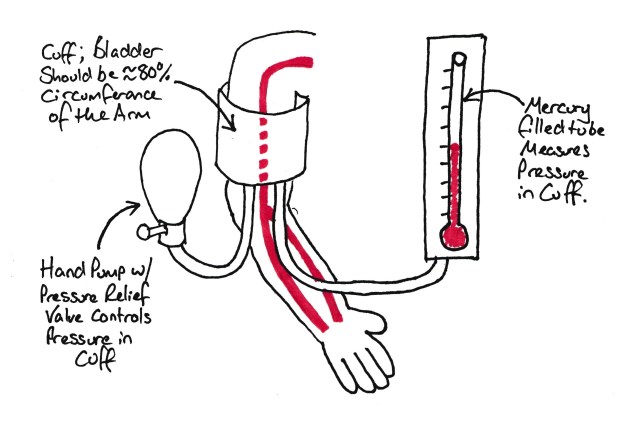
Simple sphygmomanometer.
You can feel small pulsations when you place your finger over an artery due to the variations in pressure and flow through the artery with systole and diastole. The cuff around the arm compresses the bronchial artery. When we increase the pressure within this cuff, the pressure will eventually exceed systolic pressure and these pulsations will stop. As we gradually decrease the pressure the pulsations will increase in amplitude, the maximum amplitude is equivalent to the mean arterial pressure (MAP). As we decrease the pressure further these pulsations settle to a steady level (they never entirely disappear). The point they reach the minimal amplitude is the diastolic pressure.
Now these changes will also create sound. This is because compression of a tube induces turbulent flow which is inherently noisy. The changes in sound heard distal to the cuff are called the ‘Korotkoff sounds’.
The automated machines that we use in day to day practice (‘Dynamap’) use the principles above. The machine is controlled by computer which inflates the cuff to above predicted systolic pressure. The machine then measures for small fluctuations in pressure in the cuff caused by the underlying artery. It is looking for these pulsations to cease. The pressure at which they cease is the systolic pressure. The machine then drops the pressure in the cuff in a stepwise fashion (this is audible as a quiet whoosh every second or so). It looks for the pulsations to return and measures their amplitude. This is done by measuring variations in cuff pressure with the heart beat. Remember the pulsations in the artery will be transmitted into the cuff. The MAP is the point at which these pulsations have the highest amplitude. As the pressure drops, the pulsations get less and less. They never completely disappear if the cuff is still in contact with the arm, but will reach an equilibrium. Sometimes the diastolic pressure is measured by assuming that the MAP is 1/3 of the pulse pressure above diastolic pressure.
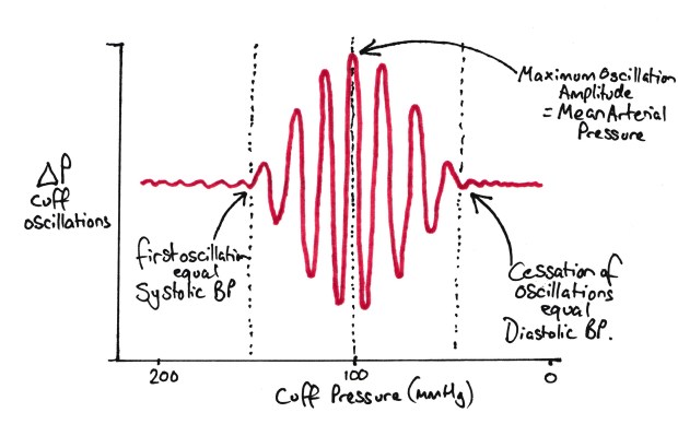
How a Dynamap works out BP
Penaz technique
Look at the pulse oximetry section before reading this, it’ll make more sense!
I doubt many people have ever seen one of these devices in action, but the college do ask about them, especially in MCQ format. The idea is that a small cuff partially occludes the artery supplying a finger. Then what is effectively a Sats/pulse oximeter probe is placed inside a cuff that is placed around a finger. The ‘sats probe’ (this is really and LED and Photodiode pair) ‘sees’ what the volume of blood is in the artery. When the volume is large, there is little light transmitted through the finger (as its absorbed by haemoglobin) and visa vera. The cuff changes in pressure to keep the volume in the artery the same (it would normally go up and down with changes in pressure during the cardiac cycle). The pressure applied to the cuff to keep the blood volume constant is then proportional to the blood pressure and hence it gives a constant read out of the pressure.
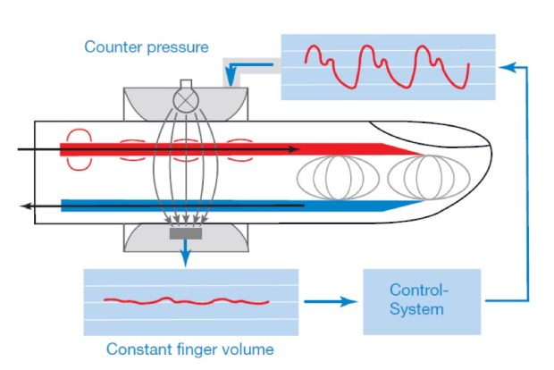
The Penaz Technique – Blood volume is kept constant, the pressure to cuff needs to apply to achieve this gives a pseudo-arterial trace – Diagram Courtesy of LiDCO
Its worth noting that LiDCO have recently released a non invasive version of the LiDCO system which uses what is effectively a Penaz type device to give an arterial trace, then applies the LiDCO algorithm to the trace to give Cardiac Output and other haemodynamic parameters. Have a look here if you want to get your geek on… (it’s a very nice device!)
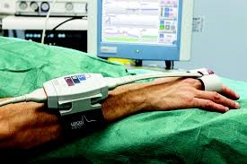
LiDCOrapid Non-Invasive BP and Cardiac Output Monitor – Courtesy of LiDCO
Direct blood pressure measurement
The Arterial Line
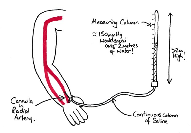
The simplest form of arterial pressure measurement
If we put a cannula into an artery and connect a column of fluid to it, we can work out the blood pressure by simply measuring the height the column rises above the level of the heart (compensating for the fluid used, e.g. mercury and mmHg vs water and cmH2O). Except that would be quite difficult to read the blood pressure due to the rapid rise and fall. Note this is just a simple manometer (see here!). Also note that you wouldn’t really use mercury in this tube due to the risk of mercury poisoning (which is nasty).
So what we do in practice is connect a transducer to the cannula with a tube of fluid between them. This allows the ability to move the transducer away from the patient and also avoids the need for a rather large manometer tube.
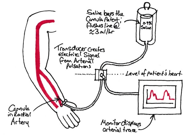
Modern invasive BP measurement
The transducer is a device which changes the pressure into a voltage which can be read by a computer. This is a combination of a strain gauge and a wheatstone bridge.
The tubing also has a flush circuit which allows flushing of the system, with a small flow constantly occurring to stop blood entering the tubing and clotting it off.
Damping & resonance
Its worth mentioning damping and resonance here. The college like this topic, so learn it well….
Resonance is the ability of an object to oscillate in response to a movement.
Think about a wine glass. If you flick it, it will make a vibrate and create a note in response to the energy you have applied to it. This is because it is resonant at that frequency. Every object has a natural resonant frequency which is the frequency which an object can resonate at with no energy needed to be applied.
Damping is the ability of an object to resist oscillation in response to a force being applied to it.
If you think of an arterial line system, sometimes the trace looks squashed or flat. This is damping coming into play. Its usually due to something highly compressible (e.g. air) or immovable (e.g. clot) in the line.
So how much damping and resonance do we want in our arterial line system?
We want the changes in BP to be accurately and rapidly recorded (to allow beat to beat measuring) but we don’t want the trace to ‘run away’ with itself and start oscillating.
If we look at an over damped trace, a step change in pressure will cause a change in the read pressure but it will be slow to react. This means that the arterial trace will not reach the maximal systolic or minimal diastolic pressure and the waveform will appear squashed. Its worth noting that the MAP is usually correct in these cases.
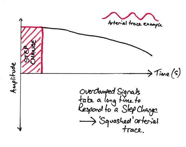
An Overdamped trace
A under damped trace will be hyper resonant and will over read any changes in the pressure. A step change will cause a rapid response, but also an overshoot in response (see graph below). An under-damped trace will over read the systolic and under read the diastolic, giving a widened pulse pressure. They can be identified by their ‘spikey’ appearance. MAP is usually accurate as well.
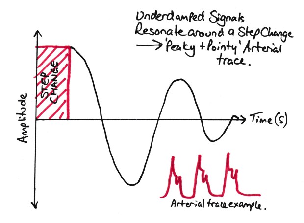
An Underdamped trace
An optimally damped trace will change in response to a step change in pressure as quickly as possible without any significant overshoot.
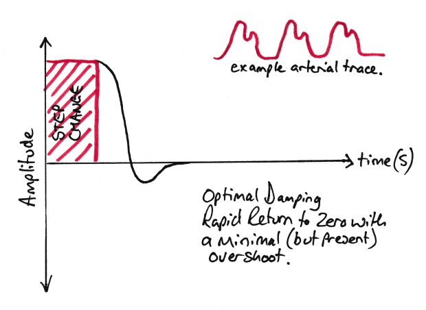
An Optimally damped trace
In terms of design of transducer systems, the advice is usually to design a device where the natural resonant frequency is over 10x higher than that you wish to measure. This means that the system is highly unlikely to resonate in response to your measured pressure change and if it does start resonating for any reason, its fairly obvious its a measurement error (ever seen a heart rate of 600+? e.g. 10 times your regular heart rate of 60). But how do we do this?
Ways to increase the resonant frequency of a system:
- Short, wide cannula
- Short, wide tubing
- Stiff material (floppy tubing makes for a damped trace)
Note, you can test the damping in your arterial line really simply. Just pull the arterial line flush for a second (MAKING SURE THE BAG HAS SALINE IN IT AND IS INFLATED!) Then observe the resultant trace. You should see one of the above waveforms (but maybe with the arterial trace on top!).
Zeroing/calibration
See this article for more information on this.
Cardiac output monitoring
Pulmonary artery catheters and pressure measurement
Although still considered the gold standard, Pulmonary artery catheters aren’t seen very often anymore, but, they are still a favourite exam topic. The examiners love pulling one out and watching the candidate squirm! They aren’t used very much any more as they are hugely invasive and if used improperly can result in patient’s death. They consist of what looks like a very long central line. These are then inserted through a wide bore sheath to allow movement of the catheter. The ‘Swan-Sheath’ has its own infusion ports and looks much like a VasCath.
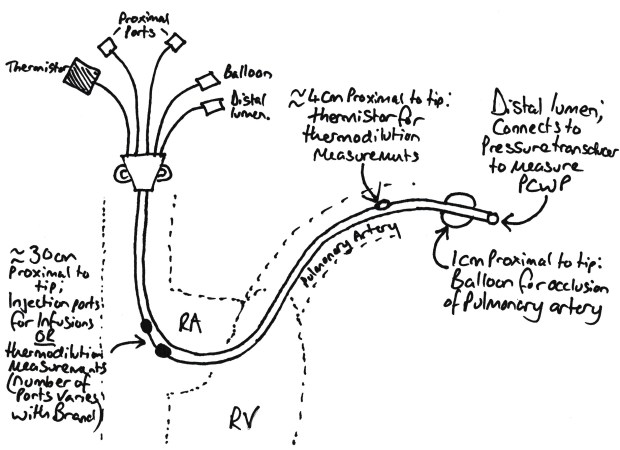
Schematic of a Swan Ganz Catheter
There are a number of things you need to be able to explain on the catheter:
- Distally there is a lumen which can be connected to a pressure transducer or taking mixed venous blood samples.
- ~1cm proximally there is a balloon which is used to occlude the pulmonary artery (more on this later).
- 4cm proximal to the tip, there is a thermistor which is used for cardiac output measurement (see below).
- 30cm proximal to the tip, there is an injection port which is used for injecting the cold fluid for cardiac output measurement.
- 31cm proximal to the tip, there is an infusion port. This is not found on all catheters.
These work by the principle of thermodilution. A cold injectate is injected into the injection port which causes a decrease in temperature of the blood circulating past it. The thermistor distally along the catheter detects this temperature change and plots it on a graph. The cardiac output is then proportional to the area under the graph.
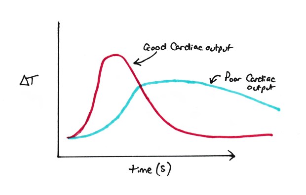
Thermodilution measurement.
Note: Be careful with this graph!!!! you’ll see this graph both like this and flipped to underneath the x axis. The graph here has ΔT as the temperature axis rather than absolute temperature, which is used when the graph is under the X axis. I think this graph is better for the pure reason everyone says that cardiac output is proportional to the area under the graph. Here it is, but with the graph under the X axis its actually the area above the line! #confused.
Now if we want to work out the ACTUAL cardiac output, we need to know a few things.
- The volume of the injectate
- The Temperature of the injectate
- The time period over which the temperature change occurs.
Then the cardiac output can be worked out using the following equation:
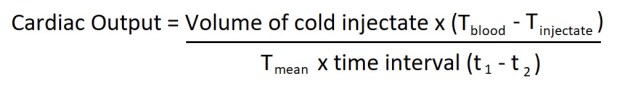
Thermodilution equation
Where:
Tblood = Blood Temperature
TInjectate = Temperature of injectate
Tmean = average temperature measured by the thermistor
T1 = when temperature drop first seen
T2 = when temperature returns to normal
To remember this, remember if you mix 10ml of liquid at 40oC with 10ml of liquid at 20oC, the eventual mix will have a temperature of 30oC. The same thing happens with cardiac output monitoring.
Example: If we inject 50ml of fluid which has a temperature 20oC less than blood into 1 litre (1000ml) of blood, it will drop the temperature by 1oC (50 x 20=1000). So, with a 50ml injectate volume at 20oC lower than blood temperature, and a cardiac output of 1L/min, we’d expect a mean temperature drop of 1oC. (these numbers aren’t real examples, its just to make the maths easy).
The only difference in cardiac output monitoring is the injectate isn’t injected into a static volume, the blood is flowing. So initially the effect is exaggerated, then gradually decreases until it stops. Hence the shape of the graph.
This gives us a static reading of cardiac output. There are two ways this can be turned into a continuous reading. One is using a catheter which has a heater proximally and a thermistor distally. The heater pulses on and off to heat the blood. This happens continuously and allows the continuous calculation. The other method uses pulse contour analysis (see below) and uses the cardiac output and arterial line trace from the ‘run’ with the cold injectate to give a baseline (ie this cardiac output gives this arterial trace) and then continuously monitor the arterial trace to deduce a continuous cardiac output reading.
Oh yeah, the Balloon. The Balloon on the Swan’ is to occlude the pulmonary artery. This then gives the transducer on the tip of the catheter an uninterrupted connection to the left atrium. This is commonly called the Pulmonary Capillary Wedge Pressure (PCWP). This can give a good measurement of function of the left side of the heart. Raised pressures quickly give rise to pulmonary oedema. Conditions which raise PCWP include: LV Failure, Aortic Stenosis/Regurgitation, Mitral Stenosis/Regurgitation. So basically anything that makes your left ventricle stop working well. PCWP can also be used to work out your pulmonary vascular resistance and hence diagnose pulmonary hypertension. Electrocardiography has generally taken over these diagnoses in recent times however.
LIDCO/PICCO
LIDCO uses the same kind of idea as a pulmonary artery catheter except from 3 things!
- Your proximal injectate port is your central line or (dependant on system) a peripheral cannula.
- Your Thermistor is changed to a lithium detection probe, usually in a modified arterial line. Usually in a large artery (Brachial or Femoral)
- Your injectate is a lithium solution.
The process is the same, inject the lithium centrally and wait for a graph to be produced. It will be slower and slightly prolonged compared to a pulmonary artery catheter but the principle is the same. The cardiac output is then worked out the same way as previously.
Be aware that LIDCO can suffer from re circulation error. This is where you get a second peak of lithium as it passes round the body for the second time. Remember temperature changes will get ‘absorbed’ into the body but the lithium isn’t absorbed quickly. To get round this, we continue the initial curve’s trajectory to zero to get what the ‘proper’ curve would look like.
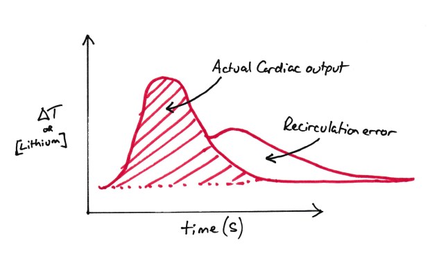
Recirculation Error
Continuous measurement is by pulse contour analysis (its coming!!) and the lithium curve is used to calibrate this.
PICCO uses the something similar to LIDCO except that the probe is a thermodilution therminstor similar to a pulmonary artery catheter.
Again, continuous measurement is by pulse contour analysis and the thermodilution curve is used to calibrate this.
Pulse Contour analysis looks at the shape of the arterial trace and uses various measurements to give an indication of cardiac output. Most of these algorithms are proprietary, so there isn’t any equations to learn as such. Just be aware that these assume a lot. They are hence probably again better for looking at trends rather than absolute figures.
There are a number of devices that rely solely on pulse contour analysis. These devices (like FloTrac and Vigileo) do not have a calibration phase like PICCO/LiDCO so are not as accurate in terms of absolute measurement. They are however useful for looking at trends and response to things like fluid therapy so still have a place in clinical use. Add this to the fact you just ‘plug and play’ into a normal arterial line and you can see their appeal.
Oesophageal Doppler
See this post to read about ultrasound and Doppler.
Doppler ultrasound can be used to measure velocity of an object quite easily. Put an ultrasound machine over any vessel and you can get a velocity reading easily. You see them on Echo reports all the time.
But, how about cardiac output?
You’ve probably seen an oesophageal Doppler at some point and been annoyed by the whooshing noises it makes. This is a little ultrasound Doppler probe on the end of a tube which is passed into the patients oesophagus, just adjacent to the descending aorta. This probe can then be positioned to give an image of the aorta.
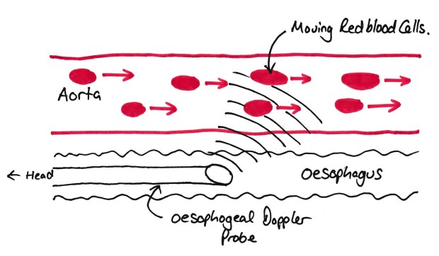
Oesophageal Doppler Probe
The important thing to note here is that the probe measures the VELOCITY of the blood in the aorta. It does NOT measure the flow of blood (examiners will pick you up on this if you say it does!). As we know from previous posts, flow is defined as the volume of fluid passing a set point per unit time. So all the probe tells us is the velocity (distance per unit time). So, we need to know the other two dimensions of the blood, as we know the length the blood is travelling per unit time.
These are worked by normograms of known aorta cross sectional areas against patient sex, age and height. The predicted cross sectional area times by the velocity will then equal the blood flow. This is then further multiplied by a constant due to some of the cardiac output not going down the descending aorta (e.g. to arms and head!).
All of these numbers (the predicted aortic cross sectional area and the constant for upper limb/head blood flow) are assumed, and hence, are a source of error. Hence oesophogeal Doppler is best used as a measure of change in cardiac output rather than looking at absolute figures.
Other sources of error with oesophogeal Doppler include:
- Movement of the probe (very annoying and does question how you can trust repeated readings when you cant be assured its moved back to the same place!)
- Diathermy!!!!! (creates noise almighty on the trace and gives you a headache if you have the sound turned on!)
Thoracic Impedance
As your heart pumps, the amount of blood within your thoracic cavity changes (increased during diastole and decreased in systole as blood is ‘ejected’ out). This will cause a change in impendence/resistance to electric current traveling across the chest. Rapid changes in this impedence associated with the heart rate can then be used to give a measure of cardiac output.
It should be noted that ventilation/breathing also causes a change in thoracic impedence (e.g. an increase in impendence on breathing in and visa versa). Most of these devices need a nice regular breathing pattern to give an accurate measure of cardiac output. This effectively limits their usage to those who are ventilated, and likely paralysed, hence their lack of widespread usage.
Random Exam factoids (i.e. the things the college like asking):
- The usual things apply here. Remember your definitions. Think of things that make good graphs for the VIVA.
- Look at all the things you measure BP with. When and why do they go wrong? Can you explain them all?
© Sam Beckett and Physics4FRCA, 2018. Unauthorized use and/or duplication of this material without express and written permission from this site’s author and/or owner is strictly prohibited.
